How DynamoDB actually works

DynamoDB makes sense the moment you stop thinking of the partition key as a column and start thinking of it as an argument to a hash function. That single value decides which physical machine your data lives on — which is why DynamoDB gives you single-digit millisecond reads at any scale, and also why a query you didn't plan for can be impossible rather than merely slow. Everything else — sort keys, indexes, the limits, the schema advice — follows from that one fact. This is the long version, because half-understanding DynamoDB is how teams end up rebuilding a table in production.

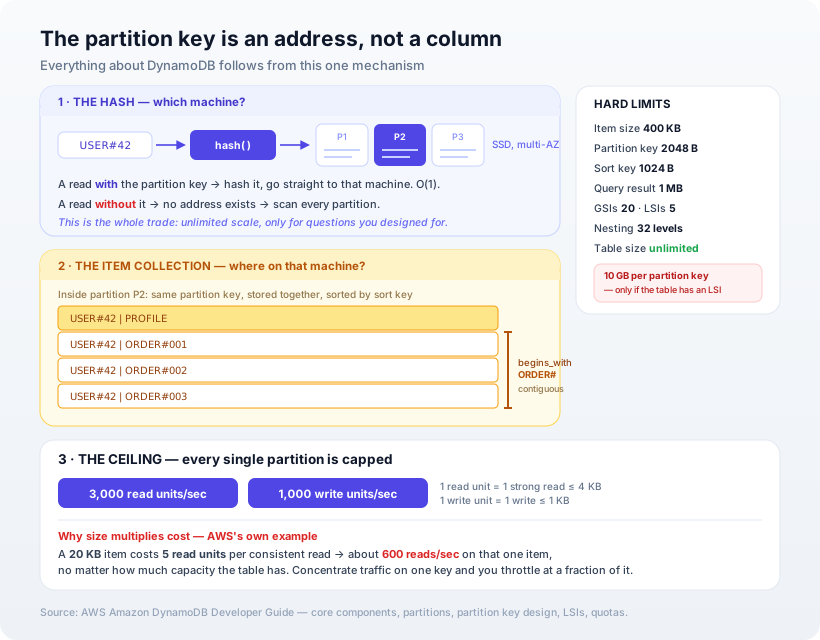
The one idea everything follows from

In Postgres, a primary key is a uniqueness constraint with an index behind it. In DynamoDB it is a storage address.

From AWS's own description: "DynamoDB uses the partition key's value as input to an internal hash function. The output from the hash function determines the partition (physical storage internal to DynamoDB) in which the item will be stored."

Read that literally. The partition key doesn't describe the item, it locates it. Which produces the defining property of the database: a read that supplies the partition key is O(1) — hash it, go to that machine, done — and a read that doesn't supply it has no address to go to, so DynamoDB must scan every partition. That's the whole trade. Constant-time access at unlimited scale, in exchange for only being able to ask questions you designed for.

There are two shapes of primary key:

• Simple — partition key only. Every partition key value is unique; one item per key.
• Composite — partition key plus sort key. Many items can share a partition key, but each must have a distinct sort key.

With a composite key, DynamoDB "tends to keep items which have the same value of partition key close together and in sorted order by the sort key." That group has a name — an item collection — and it's the unit that makes DynamoDB useful for anything beyond key-value lookups. Because the collection is stored contiguously and pre-sorted, a query like "all orders for user 42, most recent first" is a sequential read of adjacent bytes, not a search.

The partition key answers "which machine?" The sort key answers "where on that machine?" A query that can't answer the first question isn't slow — it's a table scan.

The physics: 3,000 reads and 1,000 writes

This is the number most teams never learn until an incident, and it's stated plainly in the partition key design guidance:

Every partition in a DynamoDB table is designed to deliver a maximum capacity of 3,000 read units per second and 1,000 write units per second.

The units are not requests:

• One read unit = one strongly consistent read of an item up to 4 KB. An eventually consistent read costs half a unit, so you get two of them per unit.
• One write unit = one write of an item up to 1 KB.

So item size multiplies your cost. AWS's own worked example is the clearest illustration: with a 20 KB item, a single consistent read consumes 5 read units — meaning you can drive roughly 600 consistent reads per second against that one item before hitting the partition ceiling, no matter how much capacity the table has provisioned.

This is the mechanism behind the "hot partition" problem, and why it doesn't announce itself. Your table is provisioned for 40,000 reads per second. Your traffic is well under that. But 80% of it targets one popular item — one partition key — so it lands on one partition, and that partition is capped. You get throttled at a fraction of your provisioned capacity, and the metrics that matter are the ones you weren't watching.

The fix is cardinality: AWS recommends "a partition key that can have a large number of distinct values relative to the number of items in the table," and designing "for uniform activity across all partition keys." Where a naturally hot key is unavoidable, the standard remedy is write sharding — append a suffix (POPULAR#1 … POPULAR#10) to spread one logical key across ten physical partitions, and fan the reads back in.

Indexes: two kinds, and one of them is a trap

You get two ways to query by something other than the primary key.

Global secondary index (GSI). A completely different partition key and sort key, spanning the whole table. Its keys need not be unique. It's stored separately from the base table with its own partitions and its own throughput. Default quota: 20 per table. You can add one to a live table.

Local secondary index (LSI). The same partition key as the base table, a different sort key. Limit 5 per table. Supports strongly consistent reads, which GSIs do not.

And here is the trap, stated in the LSI documentation and missed by almost everyone:

The maximum size of any item collection for a table which has one or more local secondary indexes is 10 GB.

Note the precise scope. That ceiling does not exist for tables without LSIs, and it does not apply to GSIs. Adding a single LSI imposes a hard 10 GB cap on the total data under any one partition key — base table plus all indexes combined. The reason is structural: for LSI tables, "each item collection is stored in one partition," so it inherits that partition's capacity. Without an LSI, DynamoDB "will automatically split your item collection over as many partitions as required."

Exceed it and writes to that key start failing with ItemCollectionSizeLimitExceededException. Reads still work. Deletes still work. You just can't grow.

Two more things about LSIs that catch people: they can only be created when the table is created. There is no adding one later, and no removing one without rebuilding the table. If there's any chance a partition key's data grows unbounded — a busy tenant, a chatty device, a popular forum — use a GSI.

Projections decide what's copied into an index: KEYS_ONLY, INCLUDE (named attributes), or ALL. Query an attribute you didn't project and DynamoDB performs a fetch from the base table — and you're "charged for read capacity units for every base table item fetched… for reading each entire item from the table, not just the requested attributes." A single unprojected attribute can multiply the cost of a query several times over.

How to design the schema

This is where relational instincts actively hurt, because the process runs backwards.

In Postgres you model the data and derive the queries. In DynamoDB you model the queries and derive the data.

1. Write down every access pattern first — before any table exists. Literally list them: "get user by id," "list a user's orders newest first," "find all orders in status X." This document is your schema design. If you skip it, you are guessing at hash keys.
2. Pick a partition key with high cardinality and even traffic. Not status (four values, catastrophic). Not country (skewed). Something like userId or deviceId, where no single value carries a disproportionate share of requests.
3. Use the sort key for hierarchy and ranges. Prefixed composite values (ORDER#2026-08-05#001) let one key serve several patterns: begins_with(ORDER#) for all orders, begins_with(ORDER#2026-08) for a month, between for a range. Sort keys are compared as raw UTF-8 bytes, which is why zero-padded numbers and ISO 8601 dates sort correctly and unpadded ones don't.
4. Add GSIs for the patterns the primary key can't serve — and only those. Every index costs storage and write capacity on every write.
5. Denormalise on purpose. Duplicating a user's name onto their orders isn't sloppiness here; it's how you avoid a join that doesn't exist. Accept it and own the update path.
6. Consider single-table design, but know why. Putting several entity types in one table with overloaded keys lets one query return a user and their orders in a single request. It's genuinely powerful and genuinely harder to read. Use it when you need that atomicity of access; don't adopt it as a default because it's fashionable.

Two practical notes from the docs that save real money. Attribute names are metered — they count toward storage and throughput — so st beats shipmentStatus at scale. And there is no native date type: store timestamps as epoch numbers (smaller than ISO strings, and required if you want TTL auto-deletion) or as ISO 8601 strings when human readability matters more.

The limits worth memorising

Limit	Value
Maximum item size	400 KB
Partition key value	2048 bytes
Sort key value	1024 bytes
Query result set	1 MB per request
Per-partition throughput	3,000 read units / 1,000 write units per second
GSIs per table	20 (default)
LSIs per table	5 — creatable only at table creation
Item collection (tables with an LSI only)	10 GB per partition key value
Nesting depth	32 levels
Number precision	38 digits
Table size	No practical limit

Primary key attributes must be scalar — string, number, or binary only. No maps, lists, or sets in a key.

When to use it — and when not to

DynamoDB is the right answer when:

• Your access patterns are few, well understood, and stable. Ten known queries beat "we'll figure out reporting later."
• You need predictable single-digit millisecond latency at a scale where a single Postgres instance would need sharding.
• Traffic is spiky or unpredictable, and you'd rather pay per request than provision for peak.
• The workload is key-based: sessions, user profiles, device state, event ingestion, shopping carts, leaderboards.
• You want an operational burden close to zero — no version upgrades, no vacuum, no failover drills.

Reach for Postgres instead when:

• You don't yet know all the questions you'll ask. This is most products before product-market fit, and it's the single best reason to say no.
• You need joins, ad-hoc queries, aggregates, or anything resembling reporting. SELECT ... GROUP BY has no DynamoDB equivalent that isn't a scan or a second system.
• Your data is genuinely relational — many-to-many relationships with integrity constraints.
• Your scale is ordinary. A modest Postgres box handles far more than most teams believe, and we've made that argument at length.

Our opinion

The strongest reason to choose DynamoDB is also the strongest reason to avoid it: it makes you decide your queries up front. For a team that genuinely knows its access patterns, that constraint is a gift — it forecloses the slow drift into a 40-table schema with a reporting query nobody can optimise. For a team still discovering what it's building, the same constraint is a trap, because the cost of a new question isn't a new index, it's a migration.

We'd also push back on the two most common reasons teams pick it. "It scales" is true and usually irrelevant — most products never reach a scale where Postgres is the bottleneck, and the ones that do generally have the engineering capacity to migrate when the time comes. "It's serverless so it's cheaper" is often false: at low, steady traffic a small managed Postgres instance frequently costs less than the equivalent DynamoDB table once you count indexes and their write amplification.

Where we think it's genuinely excellent is the narrow, high-volume, key-shaped workload sitting alongside a relational database — session state, rate-limit counters, device shadows, event capture. Not "our database," but "the right store for this one thing." That framing produces far better outcomes than treating the choice as an identity.

How Ashvara helps

We help teams make this decision with the access-pattern document written first, which usually settles the argument on its own — if the list is short and stable, DynamoDB is a strong candidate; if it ends with "and probably some reporting," it isn't. We also do the less glamorous work: modelling composite sort keys, sizing indexes so writes don't triple, and building the migration path for when a pattern changes.

That's core backend and API work for us, and it pairs with how we think about choosing between SQL and NoSQL generally. If you're weighing DynamoDB for something specific, tell us the queries you need to serve and we'll tell you honestly whether it fits.

---

Sources: AWS, Amazon DynamoDB Developer Guide — core components, partitions and data distribution, partition key design, local secondary indexes, data types and naming rules, and service quotas.